Here are some simulations I did for registration of 3-D Shapes

	This model is proposed in P. J. Besl and N. D. McKay. "A method for registration of 3-d shapes", IEEE Trans. Pat. Anal. and Mach. Intel. 14(2), pp 239-256, Feb 1992
	The method handles the full six degrees of freedom (rigid transformation) and is based on the iterative closest point algorithm to register two 3-D shapes.
	The point set A0 with M points from the data shape and the model shape B with N points are given. Let T0 be the initial estimate of the rigid transformation. Step 1-3 are applied for i = 1,2,3,...until convergence within a tolerance.  compute the closest point in B for each point in A(i) = T(i-1)A(i-1) (use kdtree to accelerate the speed) compute the new registration T(i) (rigid transformation) that minimizes the mean square error between point set A and its closest point set.  Apply registration to A(i).
	The first example register the red data set and the blue data set. (This is exactly the first example given in the paper)

 

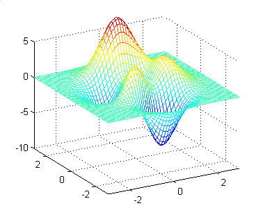
The second example: I use Delaunay triangulation and peaks function in matlab to generate the data set A (left) and mesh to generate the data set B (right). The registration result is shown in the picture in the bottom.